Hodge duality

by Stéphane Haussler

The Hodge dual is in my opinion often presented with unnecessary complexity, frequently involving from the start a number of dimensions beyond three, varying metric signatures, and a formal mathematical approach. However, the concept is intuitive in the familiar 3-dimensional Euclidean space that we experience daily. From there, generalizing the concept to 4-dimensional Minkowski space is natural.

The first part of this article presents the core intuition behind Hodge duality and is meant to be quite easy to follow. Next comes a shaping operation: Preparing the generalization to any number of dimensions and metric signatures. I lay out the relation between the exterior product, matrix determinant, surface, volume and hypervolume. This will permit to generalize the inner product to k-vectors. Finally, I systematically calculate of the Hodge duals of vectors, bivectors, trivectors and quadvectors in Minkowski spacetime with metric signature \((+,-,-,-)\). The very last step brings us to Hodge duality on k-forms based on vector/covector duality. This discussion assumes you, the reader, have a solid understanding of vector and tensor calculus, as well as familiarity with the exterior product and Élie Cartan’s differential forms.

I systematically use within this pages a toolbox of concepts and notations that I dub the Cartan-Hodge formalism. The notation is quite standard and should be widely recognized. In this page, basis vectors \(\mathbf{e}_μ\) are noted with the partial derivative symbol \(∂_μ\):

\[\begin{split}\mathbf{e}_t & = ∂_t \\ \mathbf{e}_x & = ∂_x \\ \mathbf{e}_y & = ∂_y \\ \mathbf{e}_z & = ∂_z \\\end{split}\]

I don’t necessarily expect all readers to have ever considered partial derivatives as basis vectors. For our purpose, this is simply a matter of a notation. I use for the inner product either the dot notation \(\cdot\), or the bra-ket notation from quantum mechanics \(\braket{|}\) when it helps readability [note1].

I point out the work of Michael Penn on Differential Forms . In particular, the following videos intersect greatly with the content of this page:

• Differential Forms | The Hodge operator via an inner product.

• Differential Forms | The Minkowski metric and the Hodge operator.

These videos provide an alternative, yet equivalent, approach to the conclusions presented here. There is also the added bonus that he uses the same metric signature \((+,-,-,-)\).

Duality in three dimensions

First consider a coordinate basis \(∂_x\), \(∂_y\) and \(∂_z\) in 3 dimensions corresponding to our intuitive understanding of space. Observe that we did not merely define three unit vectors, but also three unit surfaces, which we name using the wedge symbol \(∧\). The surface along the \(x\) and \(y\) axis is named \(∂_x ∧ ∂_y\), along the \(y\) and \(z\) axis \(∂_y ∧ ∂_z\), and along the \(z\) and \(x\) axis \(∂_z ∧ ∂_x\):

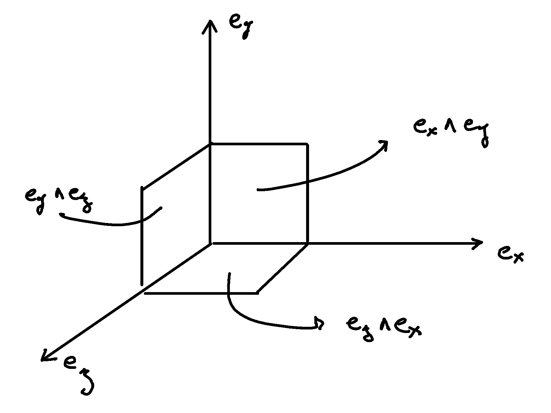
The naming of the surfaces is carefully chosen counterclock-wise. The reason is that we have not defined a mere surface from two vectors, but an oriented surface: The surface magnitude can be negative, depending on the chosen orientation. Here, we take the convention that surfaces oriented counterclockwise are positive. For example: \(∂_z ∧ ∂_x = - ∂_x ∧ ∂_z\).

Remark that we have not only decided on a naming convention, but created new mathematical objects built from two vectors and a new product denoted with the wedge symbol \(∧\). We call these objects bivectors, and the new product denoted with the wedge symbol \(∧\) exterior product. The fundamental property of these objects is that they are antisymmetric, and is already given by the discussion about the surface orientation:

\[∂_i ∧ ∂_j = - ∂_j ∧ ∂_i\]

Necessarily, \(∂_i ∧ ∂_i = 0\) since two copies of the same vectors cannot generate a surface. This can also be determined from the antisymmetric property above.

In 3 dimensions, we note that each basis bivector can be associated with a unique basis vector:

\[\begin{split}∂_x ∧ ∂_y \rightarrow ∂_z \\ ∂_y ∧ ∂_z \rightarrow ∂_x \\ ∂_z ∧ ∂_x \rightarrow ∂_y \\\end{split}\]

We note this relation with the star symbol \(⋆\):

\[\begin{split}⋆ ∂_x ∧ ∂_y = ∂_z \\ ⋆ ∂_y ∧ ∂_z = ∂_x \\ ⋆ ∂_z ∧ ∂_x = ∂_y \\\end{split}\]

This association defines a unique vector dual to every oriented surfaces called the Hodge dual. Hodge duality is noted with the star symbol \(⋆\), called the Hodge star operator. The relation holds in both direction:

\[\begin{split}⋆ ∂_z = ∂_x ∧ ∂_y \\ ⋆ ∂_x = ∂_y ∧ ∂_z \\ ⋆ ∂_y = ∂_z ∧ ∂_x \\\end{split}\]

The Hodge dual in three dimensions is the cross product. The cross product defines a vector perpendicular to the surface whose length is proportional to the amount of rotation:

\[\begin{split}∂_x ⨯ ∂_y = ⋆ ∂_x ∧ ∂_y = ∂_z \\ ∂_y ⨯ ∂_z = ⋆ ∂_y ∧ ∂_z = ∂_x \\ ∂_z ⨯ ∂_x = ⋆ ∂_z ∧ ∂_x = ∂_y \\\end{split}\]

This establishes the deep connection between the Hodge dual, rotations, surfaces, and the cross product.

Going one step futher, we observe that we did not merely define unit surfaces, but also unit volumes that we note \(∂_x ∧ ∂_y ∧ ∂_z\). We can associate the unit volume with numbers:

\[⋆ \mathbf{1} = ∂_x ∧ ∂_y ∧ ∂_z\]

As well as:

\[⋆ ∂_x ∧ ∂_y ∧ ∂_z = \mathbf{1}\]

Where \(\mathbf{1}\) is the unit number. In other words any number can be expressed as a linear combination of \(1\).

Pseudo-vectors and pseudo-scalars

As a side quest which may be of particular interest to particle physicist, I discuss the naming pseudo-vector and pseudo-scalar. From the vector basis, we have constructed with the following objects:

• scalars,

• vectors,

• bivectors corresponding to oriented surfaces, and

• trivectors corresponding to oriented volumes.

Place these objects in front of a mirror as a Gedankenexperiment. Observe the image of these objects and notice that:

• scalars are unchanged,

• vectors are unchanged,

• oriented surfaces defined from two vectors are flipped with a change of sign, and

• oriented volumes defined as trivectors (i.e. from an oriented surface and a vector) are also flipped with a change of sign.

This is the reason for the name pseudo-vector. These objects look like and nearly behave like the vectors they are associated to through Hodge duality. However and contrary to vectors, the sign of the image of a positive oriented surface goes to negative when placed in front of a mirror. The image of the Hodge dual vector is flipped.

This is also the reason for the name pseudo-scalar. These objects look like and nearly behave like the scalars they are associated to through Hodge duality. However and contrary to scalars, the sign of the image of a positive oriented volume goes to negative when placed in front of a mirror. The image of the Hodge dual scalar is flipped.

Inner product of k-vectors

The object of this section is to generalize the inner product from vectors to multivectors. This will be needed to generalize Hodge duality to any number of dimensions and metric signatures. Indeed, Minkowski space is characterized not only by 4 dimension, but also by the mixed metric signature \((+,-,-,-)\). Intuitively, we can guess that the inner product on multivectors should be influence by the metric signature. In turn, we can then also expect that the metric signature will play a role for Hodge duality in Minkowski space. We will see that the concept of the inner product is akin to measuring the size of shadows in one dimension, two dimensions, three dimensions, and k-dimensions in all generality.

Inner product of vectors

I expect you are very familiar with linear algebra, since you are interested in the more advanced topic of Hodge duality. I nonethelss recall what you may find obvious. The inner product of one vector onto another corresponds to the projection of one vector onto the other. In that sense, the inner product can be understood as a one-dimensional shadow:

Inner product on vectors.

For the basis vectors in flat euclidean space, we obtain:

\[∂_i \cdot ∂_j = \braket{∂_i | ∂_j} = δ_{ij}\]

For the basis 4-vectors in flat Minkowski space, we obtain:

\[∂_μ \cdot ∂_ν = \braket{∂_μ | ∂_ν} = η_{μν}\]

This is the starting point for a procedure which permits to meaningfully lift the inner product on vectors to the inner products on bivectors, trivectors, quadvectors, and in all generality to k-vectors.

Surfaces, volumes, hypervolumes, and the determinant of matrices

The next step is to highlight the link between the inner product and the determinant of matrices. I recall the relationship between the determinant, surfaces, volumes, and hypervolumes.

Surfaces and the determinant of 2x2 matrices.

The area of the surface \(S\) spanned by the parallelogram defined by a vector \(a ∂_x + b ∂_y\) and a vector \(c ∂_x + d ∂_y\) corresponds to the determinant of the \(2 \times 2\) matrice, where each column entries are the the components of the vectors.

\[\begin{split}S = \begin{vmatrix} a & c \\ b & d \\ \end{vmatrix} = ad - cb\end{split}\]

This can equivalently be achieved by calculating the exterior product of these two vectors:

\[\begin{split}S ∂_x ∧ ∂_y &= (a ∂_x + b ∂_y) ∧ (c ∂_x + d ∂_y) \\ &= (ad - bc) ∂_x ∧ ∂_y\end{split}\]

Calculation

Take the exterior product

\[\begin{split}S ∂_x ∧ ∂_y &= (a ∂_x + b ∂_y) ∧ (c ∂_x + d ∂_y) \\\end{split}\]

Distribute

\[\begin{split}S ∂_x ∧ ∂_y &= a ∂_x ∧ (c ∂_x + d ∂_y) + b ∂_y ∧ (c ∂_x + d ∂_y) \\ &= a ∂_x ∧ c ∂_x + a ∂_x ∧ d ∂_y + b ∂_y ∧ c ∂_x + b ∂_y ∧ d ∂_y \\\end{split}\]

Remove zero terms and take the factors in front of expression

\[\begin{split}S ∂_x ∧ ∂_y &= a ∂_x ∧ d ∂_y + b ∂_y ∧ c ∂_x \\ &= a d ∂_x ∧ ∂_y + b c ∂_y ∧ ∂_x \\\end{split}\]

Reorganize and conclude

\[\begin{split}S ∂_x ∧ ∂_y &= a d ∂_x ∧ ∂_y - b c ∂_x ∧ ∂_y \\ &= (ad - bc) ∂_x ∧ ∂_y \\\end{split}\]

Calculation in free matrix representation

Using the free matrix representation from the Cartan-Hodge formalism helps organize calculations and yields the same result.

Take the exterior product

\[\begin{split}S ∂_x ∧ ∂_y = \begin{bmatrix} a ∂_x \\ b ∂_y \\ \end{bmatrix} ∧ \begin{bmatrix} c ∂_x \\ d ∂_y \\ \end{bmatrix}\end{split}\]

Distribute and remove zero terms

\[\begin{split}S ∂_x ∧ ∂_y = \begin{bmatrix} a ∂_x ∧ d ∂_y \\ a ∂_x ∧ c ∂_x \\ b ∂_y ∧ c ∂_x \\ b ∂_y ∧ d ∂_y \end{bmatrix} = \begin{bmatrix} a ∂_x ∧ d ∂_y \\ b ∂_y ∧ c ∂_x \\ \end{bmatrix}\end{split}\]

Reorganize and conclude

\[\begin{split}S ∂_x ∧ ∂_y = \begin{bmatrix} + a d ∂_x ∧ ∂_y \\ - b c ∂_x ∧ ∂_y \\ \end{bmatrix} = (ad - bc) ∂_x ∧ ∂_y\\\end{split}\]

The same can be done to calculate the volume \(V\) of a parallelepiped defined by three vectors.

Volumes and the determinant of 3x3 matrices.

• \(r_1 = a ∂_x + b ∂_y + c ∂_z\)

• \(r_2 = u ∂_x + v ∂_y + w ∂_z\)

• \(r_3 = p ∂_x + q ∂_y + r ∂_z\)

The entries of each columns are the vector components:

\[\begin{split}V &= \begin{vmatrix} a & u & p \\ b & v & q \\ c & w & r \\ \end{vmatrix}\end{split}\]

\[\begin{split}V = + a \begin{vmatrix} v & q \\ w & r \\ \end{vmatrix} - b \begin{vmatrix} u & p \\ w & r \\ \end{vmatrix} + c \begin{vmatrix} u & p \\ v & q \\ \end{vmatrix}\end{split}\]

\[V = + avr - awq - bur + bwp + cuq - cvp\]

The above result can be equivalently achieved by taking the exterior product of these three vectors:

\[V ∂_x ∧ ∂_y ∧ ∂_z = (+avr -awq -bur +bwp +cuq -cvp) ∂_x ∧ ∂_y ∧ ∂_z\]

Calculation

Wedge the three vectors defining the volume

\[\begin{split}V ∂_x ∧ ∂_y ∧ ∂_z = \begin{bmatrix} a ∂_x \\ b ∂_y \\ c ∂_z \end{bmatrix} ∧ \begin{bmatrix} u ∂_x \\ v ∂_y \\ w ∂_z \end{bmatrix} ∧ \begin{bmatrix} p ∂_x \\ q ∂_y \\ r ∂_z \end{bmatrix}\end{split}\]

Expand the first two vectors

\[\begin{split}V ∂_x ∧ ∂_y ∧ ∂_z = \begin{bmatrix} av ∂_x ∧ ∂_y \\ aw ∂_x ∧ ∂_z \\ bu ∂_y ∧ ∂_x \\ bw ∂_y ∧ ∂_z \\ cu ∂_z ∧ ∂_x \\ cv ∂_z ∧ ∂_y \end{bmatrix} ∧ \begin{bmatrix} p ∂_x \\ q ∂_y \\ r ∂_z \end{bmatrix}\end{split}\]

Expand with the third vector

\[\begin{split}V ∂_x ∧ ∂_y ∧ ∂_z = \begin{bmatrix} avr ∂_x ∧ ∂_y ∧ ∂_z \\ awq ∂_x ∧ ∂_z ∧ ∂_y \\ bur ∂_y ∧ ∂_x ∧ ∂_z \\ bwp ∂_y ∧ ∂_z ∧ ∂_x \\ cuq ∂_z ∧ ∂_x ∧ ∂_y \\ cvp ∂_z ∧ ∂_y ∧ ∂_x \end{bmatrix}\end{split}\]

Reorder

\[\begin{split}V ∂_x ∧ ∂_y ∧ ∂_z = \begin{bmatrix} +avr ∂_x ∧ ∂_y ∧ ∂_z \\ -awq ∂_x ∧ ∂_y ∧ ∂_z \\ -bur ∂_x ∧ ∂_y ∧ ∂_z \\ +bwp ∂_x ∧ ∂_y ∧ ∂_z \\ +cuq ∂_x ∧ ∂_y ∧ ∂_z \\ -cvp ∂_x ∧ ∂_y ∧ ∂_z \end{bmatrix}\end{split}\]

Conclude

\[V ∂_x ∧ ∂_y ∧ ∂_z = (+avr -awq -bur +bwp +cuq -cvp) ∂_x ∧ ∂_y ∧ ∂_z\]

This procedure can be generalized to hypervolumes constructed from k-vectors/ The hypervolume is calculated with the determinant of a \(k \times k\) matrice, or equivalently by taking the exterior product of k k-vectors.

Inner product of vectors, bivectors, and trivectors in 3-dimensional Euclidean space

In essence, the inner product can be understood as the concept of measuring shadows. The inner product between two vectors is the measure of the 1-dimensional shadow of one vector onto the other. Similarly, the inner product between bivectors is the measure of the surface shadow of one surface onto the other. This 2-dimensional surface can be calculated from the determinant of a \(2 ⨯ 2\) matrix. We then generalize to 3-dimensions by calculating the determinant of \(3 ⨯ 3\) matrices, corresponding to the volumes covered by 3-vectors. One step further, a k-dimensional shadow measure can then be calculated using \(k ⨯ k\) matrices, corresponding to hypervolumes of dimension k. This permits to find a meaningfull way to lift the inner product from vectors to bivectors, trivectors, and k-vectors. Lifting the inner product permits to generalize the the Hodge dual to any metric signature, and apply to Minkowski space with metric signature \((+,-,-,-)\). In 3-dimensional Euclidean space, the inner product of the basis vectors, denoted with either the dot symbol \(\cdot\) or the bracket symbol \(\braket{|}\) is given by:

\[∂_i \cdot ∂_j = \braket{∂_i|∂_j} = δ_{ij}\]

Fully expanded, we have the following dot products for each basis vector combination:

Inner product of vectors

\[\begin{split}\begin{array}{c|ccc} & ∂_x & ∂_y & ∂_z \\ \hline ∂_x & 1 & 0 & 0 \\ ∂_y & 0 & 1 & 0 \\ ∂_z & 0 & 0 & 1 \\ \end{array}\end{split}\]

A first hint that the inner product can be naturally generalized to surfaces, is that in 3 dimensions, we can associate a basis surface to each of the basis vectors through the Hodge dual, as argued at the beginning of this article. It may then feel natural, since \(∂_x\) is associated to \(∂_y ∧ ∂_z\), to expect that the inner product \(\braket{∂_x|∂_x}=1\) implies that \(\braket{∂_y ∧ ∂_z | ∂_y ∧ ∂_z}=1\).

Let us consider two vectors \(a^♯\) and \(b^♯\) in 3-dimensional Euclidean space, written in component form as:

• \(a^♯ = p \, ∂_x + q \, ∂_y + r \, ∂_z\)

• \(b^♯ = u \, ∂_x + v \, ∂_y + w \, ∂_z\)

Now consider the components of \(a^♯\) and \(b^♯\) along the unit vectors \(∂_x\) and \(∂_y\):

• \(p \, ∂_x + q \, ∂_y\)

• \(u \, ∂_x + v \, ∂_y\)

The measure of the amount of shadow of the surface determined by vectors \(a^♯\) and \(b^♯\) on the \(∂_x ∧ ∂_y\) plane is the inner product on bivectors. This lifts the inner product from vectors to bivectors through the determinant:

\[\begin{split}\braket{α^♯ ∧ β^♯ | ∂_x ∧ ∂_y} = \begin{vmatrix} p & u \\ q & v \\ \end{vmatrix} = pv - qu\end{split}\]

In the same manner we obtain:

\[\begin{split}\braket{α^♯ ∧ β^♯ | ∂_y ∧ ∂_z} = \begin{vmatrix} q & v \\ r & w \\ \end{vmatrix} = qw - rv\end{split}\]

\[\begin{split}\braket{α^♯ ∧ β^♯ | ∂_z ∧ ∂_x} = \begin{vmatrix} r & w \\ p & u \\ \end{vmatrix} = ru - pw\end{split}\]

With this quantities, we have measured the amount of shadow from the surface determined by vectors \(a^♯\) and \(b^♯\) onto the unit bivectors \(∂_y ∧ ∂_z\), \(∂_z ∧ ∂_x\), and \(∂_x ∧ ∂_y\), . We can modify the expressions slightly in order to relate the vector components to the inner product of vectors. Vector components can be obtained by doting the vectors with the basis vectors:

\[\begin{split}\braket{a^♯ ∧ b^♯ | ∂_y ∧ ∂_z} = \begin{vmatrix} q & v \\ r & w \\ \end{vmatrix} = \begin{vmatrix} \braket{a^♯ | ∂_y} & \braket{b^♯ | ∂_y} \\ \braket{a^♯ | ∂_z} & \braket{b^♯ | ∂_z} \\ \end{vmatrix}\end{split}\]

\[\begin{split}\braket{a^♯ ∧ b^♯ | ∂_z ∧ ∂_x} = \begin{vmatrix} r & w \\ p & u \\ \end{vmatrix} = \begin{vmatrix} \braket{a^♯ | ∂_z} & \braket{b^♯ | ∂_z} \\ \braket{a^♯ | ∂_x} & \braket{b^♯ | ∂_x} \\ \end{vmatrix}\end{split}\]

\[\begin{split}\braket{a^♯ ∧ b^♯ | ∂_x ∧ ∂_y} = \begin{vmatrix} p & u \\ q & v \\ \end{vmatrix} = \begin{vmatrix} \braket{a^♯ | ∂_x} & \braket{b^♯ | ∂_x} \\ \braket{a^♯ | ∂_y} & \braket{b^♯ | ∂_y} \\ \end{vmatrix}\end{split}\]

Put together in condensed form:

\[\begin{split}\braket{a^♯ ∧ b^♯ | ∂_k ∧ ∂_l} = \begin{vmatrix} \braket{a^♯ | ∂_k} & \braket{b^♯ | ∂_k} \\ \braket{a^♯ | ∂_l} & \braket{b^♯ | ∂_l} \\ \end{vmatrix}\end{split}\]

With this, we can determine the surface of any arbitrary bivector compared to the basis bivectors. In particular We can replace vectors \(a^♯\) and \(b^♯\) with any of the basis vectors \(∂_x\), \(∂_y\), or \(∂_z\). We now have a technique to determine the inner product of basis bivectors:

\[\begin{split}\braket{∂_i ∧ ∂_j | ∂_k ∧ ∂_l} = \begin{vmatrix} \braket{∂_i | ∂_k} & \braket{∂_j | ∂_k} \\ \braket{∂_i | ∂_l} & \braket{∂_j | ∂_l} \\ \end{vmatrix}\end{split}\]

Which permits to obtain:

\[\begin{split}\braket{∂_y ∧ ∂_z | ∂_y ∧ ∂_z} = \begin{vmatrix} \braket{∂_y | ∂_y} & \braket{∂_z | ∂_y} \\ \braket{∂_y | ∂_z} & \braket{∂_z | ∂_z} \\ \end{vmatrix} = \begin{vmatrix} 1 & 0 \\ 0 & 1 \\ \end{vmatrix} =1\end{split}\]

\[\begin{split}\braket{∂_z ∧ ∂_x | ∂_z ∧ ∂_x} = \begin{vmatrix} \braket{∂_z | ∂_z} & \braket{∂_x | ∂_z} \\ \braket{∂_z | ∂_x} & \braket{∂_x | ∂_x} \\ \end{vmatrix} = \begin{vmatrix} 1 & 0 \\ 0 & 1 \\ \end{vmatrix} = 1\end{split}\]

\[\begin{split}\braket{∂_x ∧ ∂_y | ∂_x ∧ ∂_y} = \begin{vmatrix} \braket{∂_x | ∂_x} & \braket{∂_y | ∂_x} \\ \braket{∂_x | ∂_y} & \braket{∂_y | ∂_y} \\ \end{vmatrix} = \begin{vmatrix} 1 & 0 \\ 0 & 1 \\ \end{vmatrix} = 1\end{split}\]

All other inner products are zero. For example:

\[\begin{split}\braket{∂_y ∧ ∂_z | ∂_x ∧ ∂_y} = \begin{vmatrix} \braket{∂_y | ∂_x} & \braket{∂_z | ∂_x} \\ \braket{∂_y | ∂_y} & \braket{∂_z | ∂_y} \\ \end{vmatrix} = \begin{vmatrix} 0 & 0 \\ 0 & 0 \\ \end{vmatrix} = 0\end{split}\]

In summary, we obtain:

Inner product of bivectors

\[\begin{split}\begin{array}{c|cccc} & ∂_y ∧ ∂_z & ∂_z ∧ ∂_x & ∂_x ∧ ∂_y \\ \hline ∂_y ∧ ∂_z & 1 & 0 & 0 \\ ∂_z ∧ ∂_x & 0 & 1 & 0 \\ ∂_x ∧ ∂_y & 0 & 0 & 1 \\ \end{array}\end{split}\]

Finally, we generalize lifting the inner product to trivectors. In 3-dimensional Euclidean space, we get for the unit trivector:

\[\begin{split}\braket{∂_x ∧ ∂_y ∧ ∂_z | ∂_x ∧ ∂_y ∧ ∂_z} = \begin{vmatrix} \braket{∂_x | ∂_x} & \braket{∂_y | ∂_x} & \braket{∂_z | ∂_x}\\ \braket{∂_x | ∂_y} & \braket{∂_y | ∂_y} & \braket{∂_z | ∂_y}\\ \braket{∂_x | ∂_z} & \braket{∂_y | ∂_z} & \braket{∂_z | ∂_z}\\ \end{vmatrix}\end{split}\]

\[\begin{split}\braket{∂_x ∧ ∂_y ∧ ∂_z | ∂_x ∧ ∂_y ∧ ∂_z} = \begin{vmatrix} 1 & 0 & 0\\ 0 & 1 & 0\\ 0 & 0 & 1\\ \end{vmatrix}\end{split}\]

\[\braket{∂_x ∧ ∂_y ∧ ∂_z | ∂_x ∧ ∂_y ∧ ∂_z} = 1\]

In table form, we have:

Inner product of trivectors

\[\begin{split}\begin{array}{c|c} & ∂_x ∧ ∂_y ∧ ∂_z \\ \hline ∂_x ∧ ∂_y ∧ ∂_z & 1 \\ \end{array}\end{split}\]

With this, we remark we have found a meaningfull and reasonable way to extend the inner product to k-forms in Minkowski space. This approach is meaningful, as the inner product of the basis vectors inherently incorporates the metric signature.

Inner product of k-vectors in Minkowski space

The inner product in Minkowski space of the basis vectors is:

\[∂_μ \cdot ∂_ν = \braket{∂_μ|∂_ν} = η_{μν}\]

Fully expanded in table form we have:

Inner product of vectors in Minkowski space

\[\begin{split}\begin{array}{c|rrrr} & ∂_t & ∂_x & ∂_y & ∂_z \\ \hline ∂_t & +1 & 0 & 0 & 0 \\ ∂_x & 0 & -1 & 0 & 0 \\ ∂_y & 0 & 0 & -1 & 0 \\ ∂_z & 0 & 0 & 0 & -1 \\ \end{array}\end{split}\]

We use our procedure for lifting the inner product to bivectors:

\[\begin{split}\braket{∂_μ ∧ ∂_ν | ∂_ρ ∧ ∂_σ} = \begin{vmatrix} ∂_μ \cdot ∂_ρ & ∂_ν \cdot ∂_ρ \\ ∂_μ \cdot ∂_σ & ∂_ν \cdot ∂_σ \\ \end{vmatrix}\end{split}\]

We get in table form:

Inner product of bivectors in Minkowski space

\[\begin{split}\begin{array}{c|rrrrrr} & ∂_t ∧ ∂_x & ∂_t ∧ ∂_y & ∂_t ∧ ∂_z & ∂_y ∧ ∂_z & ∂_z ∧ ∂_x & ∂_x ∧ ∂_y \\ \hline ∂_t ∧ ∂_x & -1 & 0 & 0 & 0 & 0 & 0 \\ ∂_t ∧ ∂_y & 0 & -1 & 0 & 0 & 0 & 0 \\ ∂_t ∧ ∂_z & 0 & 0 & -1 & 0 & 0 & 0 \\ ∂_y ∧ ∂_z & 0 & 0 & 0 & +1 & 0 & 0 \\ ∂_z ∧ ∂_x & 0 & 0 & 0 & 0 & +1 & 0 \\ ∂_x ∧ ∂_y & 0 & 0 & 0 & 0 & 0 & +1 \\ \end{array}\end{split}\]

Calculations

In this dropdown section, I extend the inner product to all non-zero bivector combinations and provide an example of a zero combination.

Basis bivectors involving the temporal dimension

\[\begin{split}\braket{∂_t ∧ ∂_x | ∂_t ∧ ∂_x} = \begin{vmatrix} ∂_t \cdot ∂_t & ∂_x \cdot ∂_t \\ ∂_t \cdot ∂_x & ∂_x \cdot ∂_x \\ \end{vmatrix} = \begin{vmatrix} \begin{alignedat}{3} + & 1 & \; & 0 \\ & 0 & \; - & 1 \\ \end{alignedat} \end{vmatrix} = -1\end{split}\]

\[\begin{split}\braket{∂_t ∧ ∂_y | ∂_t ∧ ∂_y} = \begin{vmatrix} ∂_t \cdot ∂_t & ∂_y \cdot ∂_t \\ ∂_t \cdot ∂_y & ∂_y \cdot ∂_y \\ \end{vmatrix} = \begin{vmatrix} \begin{alignedat}{3} + & 1 & \; & 0 \\ & 0 & \; - & 1 \\ \end{alignedat} \end{vmatrix} = -1\end{split}\]

\[\begin{split}\braket{∂_t ∧ ∂_z | ∂_t ∧ ∂_z} = \begin{vmatrix} ∂_t \cdot ∂_t & ∂_z \cdot ∂_t \\ ∂_t \cdot ∂_z & ∂_z \cdot ∂_z \\ \end{vmatrix} = \begin{vmatrix} \begin{alignedat}{3} + & 1 & \; & 0 \\ & 0 & \; - & 1 \\ \end{alignedat} \end{vmatrix} = -1\end{split}\]

Basis bivectors involving the spatial dimensions

\[\begin{split}\braket{∂_y ∧ ∂_z | ∂_y ∧ ∂_z} = \begin{vmatrix} ∂_y \cdot ∂_y & ∂_z \cdot ∂_y \\ ∂_y \cdot ∂_z & ∂_z \cdot ∂_z \\ \end{vmatrix} = \begin{vmatrix} \begin{alignedat}{3} - & 1 & \; & 0 \\ & 0 & \; - & 1 \\ \end{alignedat} \end{vmatrix} = +1\end{split}\]

\[\begin{split}\braket{∂_z ∧ ∂_x | ∂_z ∧ ∂_x} = \begin{vmatrix} ∂_z \cdot ∂_z & ∂_x \cdot ∂_z \\ ∂_z \cdot ∂_x & ∂_x \cdot ∂_x \\ \end{vmatrix} = \begin{vmatrix} \begin{alignedat}{3} - & 1 & \; & 0 \\ & 0 & \; - & 1 \\ \end{alignedat} \end{vmatrix} = +1\end{split}\]

\[\begin{split}\braket{∂_x ∧ ∂_y | ∂_x ∧ ∂_y} = \begin{vmatrix} ∂_x \cdot ∂_x & ∂_y \cdot ∂_x \\ ∂_x \cdot ∂_y & ∂_y \cdot ∂_y \\ \end{vmatrix} = \begin{vmatrix} \begin{alignedat}{3} - & 1 & \; & 0 \\ & 0 & \; - & 1 \\ \end{alignedat} \end{vmatrix} = +1\end{split}\]

Basis vectors resulting in zero inner products

All other inner products are zero. I demonstrate one example calculation, assuming the remaining cases will be clear to the reader.

\[\begin{split}\braket{∂_t ∧ ∂_x | ∂_x ∧ ∂_y} = \begin{vmatrix} ∂_t \cdot ∂_x & ∂_x \cdot ∂_x \\ ∂_t \cdot ∂_y & ∂_x \cdot ∂_y \\ \end{vmatrix} = \begin{vmatrix} \begin{alignedat}{3} & 0 & \; + & 1 \\ & 0 & \; & 0 \\ \end{alignedat} \end{vmatrix} = 0\end{split}\]

As well as for trivectors:

\[\begin{split}\braket{∂_μ ∧ ∂_ν ∧ ∂_λ | ∂_ρ ∧ ∂_σ ∧ ∂_τ} = \begin{vmatrix} ∂_μ \cdot ∂_ρ & ∂_ν \cdot ∂_ρ & ∂_λ \cdot ∂_ρ \\ ∂_μ \cdot ∂_σ & ∂_ν \cdot ∂_σ & ∂_λ \cdot ∂_σ \\ ∂_μ \cdot ∂_τ & ∂_ν \cdot ∂_τ & ∂_λ \cdot ∂_τ \\ \end{vmatrix}\end{split}\]

Inner product of trivectors in Minkowski space

\[\begin{split}\begin{array}{c|rrrr} & ∂_x ∧ ∂_y ∧ ∂_z & ∂_t ∧ ∂_y ∧ ∂_z & ∂_t ∧ ∂_z ∧ ∂_x & ∂_t ∧ ∂_x ∧ ∂_y \\ \hline ∂_x ∧ ∂_y ∧ ∂_z & -1 & 0 & 0 & 0 \\ ∂_t ∧ ∂_y ∧ ∂_z & 0 & +1 & 0 & 0 \\ ∂_t ∧ ∂_z ∧ ∂_x & 0 & 0 & +1 & 0 \\ ∂_t ∧ ∂_x ∧ ∂_y & 0 & 0 & 0 & +1 \\ \end{array}\end{split}\]

Calculations

\[\begin{split}\braket{∂_x ∧ ∂_y ∧ ∂_z | ∂_x ∧ ∂_y ∧ ∂_z} = \begin{vmatrix} ∂_x \cdot ∂_x & ∂_y \cdot ∂_x & ∂_z \cdot ∂_x \\ ∂_x \cdot ∂_y & ∂_y \cdot ∂_y & ∂_z \cdot ∂_y \\ ∂_x \cdot ∂_z & ∂_y \cdot ∂_z & ∂_z \cdot ∂_z \\ \end{vmatrix} = \begin{vmatrix} -1 & 0 & 0 \\ 0 & -1 & 0 \\ 0 & 0 & -1 \\ \end{vmatrix} = -1\end{split}\]

\[\begin{split}\braket{∂_t ∧ ∂_y ∧ ∂_z | ∂_t ∧ ∂_y ∧ ∂_z} = \begin{vmatrix} ∂_t \cdot ∂_t & ∂_y \cdot ∂_t & ∂_z \cdot ∂_t \\ ∂_t \cdot ∂_y & ∂_y \cdot ∂_y & ∂_z \cdot ∂_y \\ ∂_t \cdot ∂_z & ∂_y \cdot ∂_z & ∂_z \cdot ∂_z \\ \end{vmatrix} = \begin{vmatrix} +1 & 0 & 0 \\ 0 & -1 & 0 \\ 0 & 0 & -1 \\ \end{vmatrix} = 1\end{split}\]

\[\begin{split}\braket{∂_t ∧ ∂_z ∧ ∂_x | ∂_t ∧ ∂_z ∧ ∂_x} = \begin{vmatrix} ∂_t \cdot ∂_t & ∂_z \cdot ∂_t & ∂_x \cdot ∂_t \\ ∂_t \cdot ∂_z & ∂_z \cdot ∂_z & ∂_x \cdot ∂_z \\ ∂_t \cdot ∂_x & ∂_z \cdot ∂_x & ∂_x \cdot ∂_x \\ \end{vmatrix} = \begin{vmatrix} +1 & 0 & 0 \\ 0 & -1 & 0 \\ 0 & 0 & -1 \\ \end{vmatrix} = 1\end{split}\]

\[\begin{split}\braket{∂_t ∧ ∂_x ∧ ∂_y | ∂_t ∧ ∂_x ∧ ∂_y} = \begin{vmatrix} ∂_t \cdot ∂_t & ∂_x \cdot ∂_t & ∂_y \cdot ∂_t \\ ∂_t \cdot ∂_x & ∂_x \cdot ∂_x & ∂_y \cdot ∂_x \\ ∂_t \cdot ∂_y & ∂_x \cdot ∂_y & ∂_y \cdot ∂_y \\ \end{vmatrix} = \begin{vmatrix} +1 & 0 & 0 \\ 0 & -1 & 0 \\ 0 & 0 & -1 \\ \end{vmatrix} = 1\end{split}\]

In Minkowski space, all quadvectors are proportional to \(∂_t ∧ ∂_x ∧ ∂_y ∧ ∂_z\):

\[\begin{split}\braket{∂_t ∧ ∂_x ∧ ∂_y ∧ ∂_z | ∂_t ∧ ∂_x ∧ ∂_y ∧ ∂_z} = \begin{vmatrix} ∂_t \cdot ∂_t & ∂_x \cdot ∂_t & ∂_y \cdot ∂_t & ∂_y \cdot ∂_t \\ ∂_t \cdot ∂_x & ∂_x \cdot ∂_x & ∂_y \cdot ∂_x & ∂_y \cdot ∂_x \\ ∂_t \cdot ∂_y & ∂_x \cdot ∂_y & ∂_y \cdot ∂_y & ∂_y \cdot ∂_y \\ ∂_t \cdot ∂_z & ∂_x \cdot ∂_z & ∂_y \cdot ∂_z & ∂_y \cdot ∂_z \\ \end{vmatrix}\end{split}\]

\[\begin{split}\braket{∂_t ∧ ∂_x ∧ ∂_y ∧ ∂_z | ∂_t ∧ ∂_x ∧ ∂_y ∧ ∂_z} = \begin{vmatrix} +1 & 0 & 0 & 0 \\ 0 & -1 & 0 & 0 \\ 0 & 0 & -1 & 0 \\ 0 & 0 & 0 & -1 \\ \end{vmatrix}\end{split}\]

\[\braket{∂_t ∧ ∂_x ∧ ∂_y ∧ ∂_z | ∂_t ∧ ∂_x ∧ ∂_y ∧ ∂_z} = -1\]

Inner product of quadvectors in Minkowski space

\[\begin{split}\begin{array}{c|c} & ∂_t ∧ ∂_x ∧ ∂_y ∧ ∂_z \\ \hline ∂_t ∧ ∂_x ∧ ∂_y ∧ ∂_z & -1 \\ \end{array}\end{split}\]

Formal and natural definition

In 3-dimensional Euclidean space, the Hodge dual of a k-vector \(β\) is uniquely defined by the property that for any other k-vector \(α\), the following property holds:

\[α ∧ ⋆ β = \braket{α | β} \; ∂_x ∧ ∂_y ∧ ∂_z\]

In essence, this asks: Given a k-vector, which m-vector fills the remaining space? Where the inner product \(\braket{α | β}\) ensures that \(⋆ β\) is unique. This question can be viewed as a natural definition and be used for practical calculations. For 4-dimensional Minkowski space, the definition is:

\[α ∧ ⋆ β = \braket{α | β} \; ∂_t ∧ ∂_x ∧ ∂_y ∧ ∂_z\]

For instance, when seeking the Hodge dual \(⋆(∂_t ∧ ∂_x)\), we know that it must be \(∂_y ∧ ∂_z\) to complete the space, with the sign determined by the inner product \(\braket{∂_t ∧ ∂_x | ∂_t ∧ ∂_x} = -1\). Therefore, in this example, we obtain:

\[⋆ ∂_t ∧ ∂_x = - ∂_y ∧ ∂_z\]

Duality in Minkowski space

k-vectors

With this, we can conclude and fully determine the Hodge dual of all k-vectors in Minkowski space:

Hodge duals of vectors in Minkowski Space

\[\begin{split}⋆ ∂_t & = ∂_x ∧ ∂_y ∧ ∂_z \\ ⋆ ∂_x & = ∂_t ∧ ∂_y ∧ ∂_z \\ ⋆ ∂_y & = ∂_t ∧ ∂_z ∧ ∂_x \\ ⋆ ∂_z & = ∂_t ∧ ∂_x ∧ ∂_y \\\end{split}\]

Calculations

Determine the Hodge duals up to the sign

To obtain the volume element \(∂_t ∧ ∂_x ∧ ∂_y ∧ ∂_z\), the Hodge duals must be proportional to:

\[\begin{split}\begin{alignedat}{2} ⋆ ∂_t & \propto & ∂_x ∧ ∂_y ∧ ∂_z \\ ⋆ ∂_x & \propto & ∂_t ∧ ∂_z ∧ ∂_y \\ ⋆ ∂_y & \propto & ∂_t ∧ ∂_x ∧ ∂_z \\ ⋆ ∂_z & \propto & ∂_t ∧ ∂_y ∧ ∂_x \\ \end{alignedat}\end{split}\]

Check the sign

Since the above was mentally determined, we check by wedging the left part to the right part of the equations above in order to make sure the sign is positive when reordered into the volume element \(∂_t ∧ ∂_x ∧ ∂_y ∧ ∂_z\).

\[\begin{split}⋆ ∂_t \propto ∂_x ∧ ∂_y ∧ ∂_z \rightarrow \phantom{-} ∂_t ∧ ∂_x ∧ ∂_y ∧ ∂_z \\\end{split}\]

\[\begin{split}\begin{alignedat}{2} ⋆ ∂_x \propto ∂_t ∧ ∂_z ∧ ∂_y \rightarrow & & ∂_x ∧ ∂_t ∧ ∂_z ∧ ∂_y \\ & - & ∂_t ∧ ∂_x ∧ ∂_z ∧ ∂_y \\ & & ∂_t ∧ ∂_x ∧ ∂_y ∧ ∂_z \\ \end{alignedat}\end{split}\]

\[\begin{split}\begin{alignedat}{2} ⋆ ∂_y \propto ∂_t ∧ ∂_x ∧ ∂_z \rightarrow & & ∂_y ∧ ∂_t ∧ ∂_x ∧ ∂_z \\ & - & ∂_t ∧ ∂_y ∧ ∂_x ∧ ∂_z \\ & - & ∂_t ∧ ∂_x ∧ ∂_y ∧ ∂_z \\ \end{alignedat}\end{split}\]

\[\begin{split}\begin{alignedat}{2} ⋆ ∂_z \propto ∂_t ∧ ∂_y ∧ ∂_x \rightarrow & & ∂_z ∧ ∂_t ∧ ∂_y ∧ ∂_x \\ & - & ∂_t ∧ ∂_z ∧ ∂_y ∧ ∂_x \\ & & ∂_t ∧ ∂_y ∧ ∂_z ∧ ∂_x \\ & - & ∂_t ∧ ∂_y ∧ ∂_x ∧ ∂_z \\ & & ∂_t ∧ ∂_x ∧ ∂_y ∧ ∂_z \\ \end{alignedat}\end{split}\]

Use the definition of the Hodge dual

\[\begin{split}\begin{alignedat}{2} ⋆ ∂_t & = \braket{∂_t | ∂_t} & ∂_x ∧ ∂_y ∧ ∂_z \\ ⋆ ∂_x & = \braket{∂_x | ∂_x} & ∂_t ∧ ∂_z ∧ ∂_y \\ ⋆ ∂_y & = \braket{∂_y | ∂_y} & ∂_t ∧ ∂_x ∧ ∂_z \\ ⋆ ∂_z & = \braket{∂_z | ∂_z} & ∂_t ∧ ∂_y ∧ ∂_x \\ \end{alignedat}\end{split}\]

Reorder

\[\begin{split}\begin{alignedat}{3} ⋆ ∂_t & = \braket{∂_t | ∂_t} & (+1) & ∂_x ∧ ∂_y ∧ ∂_z \\ ⋆ ∂_x & = \braket{∂_x | ∂_x} & (-1) & ∂_t ∧ ∂_y ∧ ∂_z \\ ⋆ ∂_y & = \braket{∂_y | ∂_y} & (-1) & ∂_t ∧ ∂_z ∧ ∂_x \\ ⋆ ∂_z & = \braket{∂_z | ∂_z} & (-1) & ∂_t ∧ ∂_x ∧ ∂_y \\ \end{alignedat}\end{split}\]

Apply the values of the inner products

\[\begin{split}\begin{alignedat}{3} ⋆ ∂_t & = (+1) & (+1) & ∂_x ∧ ∂_y ∧ ∂_z \\ ⋆ ∂_x & = (-1) & (-1) & ∂_t ∧ ∂_y ∧ ∂_z \\ ⋆ ∂_y & = (-1) & (-1) & ∂_t ∧ ∂_z ∧ ∂_x \\ ⋆ ∂_z & = (-1) & (-1) & ∂_t ∧ ∂_x ∧ ∂_y \\ \end{alignedat}\end{split}\]

Conclude

\[\begin{split}⋆ ∂_t & = ∂_x ∧ ∂_y ∧ ∂_z \\ ⋆ ∂_x & = ∂_t ∧ ∂_y ∧ ∂_z \\ ⋆ ∂_y & = ∂_t ∧ ∂_z ∧ ∂_x \\ ⋆ ∂_z & = ∂_t ∧ ∂_x ∧ ∂_y \\\end{split}\]

If you feel more comfortable with a more mechanical approach I redirect you to the video by Michael Penn: Differential Forms | The Minkowski metric and the Hodge operator.

Hodge duals of bivectors in Minkowski space

\[\begin{split}\begin{alignedat}{2} ⋆ (∂_t ∧ ∂_x) &= -& ∂_y ∧ ∂_z \\ ⋆ (∂_t ∧ ∂_y) &= -& ∂_z ∧ ∂_x \\ ⋆ (∂_t ∧ ∂_z) &= -& ∂_x ∧ ∂_y \\ ⋆ (∂_y ∧ ∂_z) &= & ∂_t ∧ ∂_x \\ ⋆ (∂_z ∧ ∂_x) &= & ∂_t ∧ ∂_y \\ ⋆ (∂_x ∧ ∂_y) &= & ∂_t ∧ ∂_z \\ \end{alignedat}\end{split}\]

Calculations

To obtain the volume element \(∂_t ∧ ∂_x ∧ ∂_y ∧ ∂_z\), the Hodge duals must be proportional to:

\[\begin{split}⋆ (∂_t ∧ ∂_x) \propto ∂_y ∧ ∂_z \\ ⋆ (∂_t ∧ ∂_y) \propto ∂_z ∧ ∂_x \\ ⋆ (∂_t ∧ ∂_z) \propto ∂_x ∧ ∂_y \\ ⋆ (∂_y ∧ ∂_z) \propto ∂_t ∧ ∂_x \\ ⋆ (∂_z ∧ ∂_x) \propto ∂_t ∧ ∂_y \\ ⋆ (∂_x ∧ ∂_y) \propto ∂_t ∧ ∂_z \\\end{split}\]

For example, taking the second entry as an example \(⋆ (∂_t ∧ ∂_y) \propto ∂_z ∧ ∂_x\), we have:

\[\begin{split}\begin{alignedat}{2} ⋆ (∂_t ∧ ∂_y) \propto ∂_z ∧ ∂_x & \rightarrow & ∂_t ∧ ∂_y ∧ ∂_z ∧ ∂_x \\ & \rightarrow - & ∂_t ∧ ∂_y ∧ ∂_x ∧ ∂_z \\ & \rightarrow & ∂_t ∧ ∂_x ∧ ∂_y ∧ ∂_z \\ \end{alignedat}\end{split}\]

Taken all together and with the inner product, we have:

\[\begin{split}⋆ (∂_t ∧ ∂_x) &= \braket{∂_t ∧ ∂_x|∂_t ∧ ∂_x} \, ∂_y ∧ ∂_z \\ ⋆ (∂_t ∧ ∂_y) &= \braket{∂_t ∧ ∂_y|∂_t ∧ ∂_y} \, ∂_z ∧ ∂_x \\ ⋆ (∂_t ∧ ∂_z) &= \braket{∂_t ∧ ∂_z|∂_t ∧ ∂_z} \, ∂_x ∧ ∂_y \\ ⋆ (∂_y ∧ ∂_z) &= \braket{∂_y ∧ ∂_z|∂_y ∧ ∂_z} \, ∂_t ∧ ∂_x \\ ⋆ (∂_z ∧ ∂_x) &= \braket{∂_z ∧ ∂_x|∂_z ∧ ∂_x} \, ∂_t ∧ ∂_y \\ ⋆ (∂_x ∧ ∂_y) &= \braket{∂_x ∧ ∂_y|∂_x ∧ ∂_y} \, ∂_t ∧ ∂_z \\\end{split}\]

Which simplifies to:

\[\begin{split}\begin{alignedat}{3} ⋆ (∂_t ∧ ∂_x) &= -& ∂_y ∧ ∂_z \\ ⋆ (∂_t ∧ ∂_y) &= -& ∂_z ∧ ∂_x \\ ⋆ (∂_t ∧ ∂_z) &= -& ∂_x ∧ ∂_y \\ ⋆ (∂_y ∧ ∂_z) &= & ∂_t ∧ ∂_x \\ ⋆ (∂_z ∧ ∂_x) &= & ∂_t ∧ ∂_y \\ ⋆ (∂_x ∧ ∂_y) &= & ∂_t ∧ ∂_z \\ \end{alignedat}\end{split}\]

Hodge duals of trivectors in Minkowski space

\[\begin{split}⋆ ∂_x ∧ ∂_y ∧ ∂_z &= ∂_t \\ ⋆ ∂_t ∧ ∂_y ∧ ∂_z &= ∂_x \\ ⋆ ∂_t ∧ ∂_z ∧ ∂_x &= ∂_y \\ ⋆ ∂_t ∧ ∂_x ∧ ∂_y &= ∂_z \\\end{split}\]

Calculations

To obtain the volume element \(∂_t ∧ ∂_x ∧ ∂_y ∧ ∂_z\), the Hodge duals must be proportional to:

\[\begin{split}\begin{alignedat}{2} ⋆ ∂_x ∧ ∂_y ∧ ∂_z &\propto - & ∂_t \\ ⋆ ∂_t ∧ ∂_y ∧ ∂_z &\propto & ∂_x \\ ⋆ ∂_t ∧ ∂_z ∧ ∂_x &\propto & ∂_y \\ ⋆ ∂_t ∧ ∂_x ∧ ∂_y &\propto & ∂_z \\ \end{alignedat}\end{split}\]

Indeed, we check this for all entries:

\[\begin{split}\begin{alignedat}{2} ⋆ ∂_x ∧ ∂_y ∧ ∂_z \propto ∂_t & \rightarrow & ∂_x ∧ ∂_y ∧ ∂_z ∧ ∂_t \\ & \rightarrow - & ∂_x ∧ ∂_y ∧ ∂_t ∧ ∂_z \\ & \rightarrow & ∂_x ∧ ∂_t ∧ ∂_y ∧ ∂_z \\ & \rightarrow - & ∂_t ∧ ∂_x ∧ ∂_y ∧ ∂_z \\ \end{alignedat}\end{split}\]

\[\begin{split}\begin{alignedat}{2} ⋆ ∂_t ∧ ∂_y ∧ ∂_z \propto ∂_x & \rightarrow & ∂_t ∧ ∂_y ∧ ∂_z ∧ ∂_x \\ & \rightarrow - & ∂_t ∧ ∂_y ∧ ∂_x ∧ ∂_z \\ & \rightarrow & ∂_t ∧ ∂_x ∧ ∂_y ∧ ∂_z \\ \end{alignedat}\end{split}\]

\[\begin{split}\begin{alignedat}{2} ⋆ ∂_t ∧ ∂_z ∧ ∂_x \propto ∂_y & \rightarrow & ∂_t ∧ ∂_z ∧ ∂_x ∧ ∂_y \\ & \rightarrow - & ∂_t ∧ ∂_x ∧ ∂_z ∧ ∂_y \\ & \rightarrow & ∂_t ∧ ∂_x ∧ ∂_y ∧ ∂_z \\ \end{alignedat}\end{split}\]

\[\begin{split}⋆ ∂_t ∧ ∂_x ∧ ∂_y \propto ∂_z \rightarrow \phantom{-} ∂_t ∧ ∂_x ∧ ∂_y ∧ ∂_z \\\end{split}\]

Taken all together and with the inner product:

\[\begin{split}\begin{alignedat}{2} ⋆ ∂_x ∧ ∂_y ∧ ∂_z &= \braket{∂_x ∧ ∂_y ∧ ∂_z | ∂_x ∧ ∂_y ∧ ∂_z}- & ∂_t \\ ⋆ ∂_t ∧ ∂_y ∧ ∂_z &= \braket{∂_t ∧ ∂_y ∧ ∂_z | ∂_t ∧ ∂_y ∧ ∂_z} & ∂_x \\ ⋆ ∂_t ∧ ∂_z ∧ ∂_x &= \braket{∂_t ∧ ∂_z ∧ ∂_x | ∂_t ∧ ∂_z ∧ ∂_x} & ∂_y \\ ⋆ ∂_t ∧ ∂_x ∧ ∂_y &= \braket{∂_t ∧ ∂_x ∧ ∂_y | ∂_t ∧ ∂_x ∧ ∂_y} & ∂_z \\ \end{alignedat}\end{split}\]

\[\begin{split}⋆ ∂_x ∧ ∂_y ∧ ∂_z &= ∂_t \\ ⋆ ∂_t ∧ ∂_y ∧ ∂_z &= ∂_x \\ ⋆ ∂_t ∧ ∂_z ∧ ∂_x &= ∂_y \\ ⋆ ∂_t ∧ ∂_x ∧ ∂_y &= ∂_z \\\end{split}\]

Hodge duals of quadvectors in Minkowski space

\[⋆ ∂_t ∧ ∂_x ∧ ∂_y ∧ ∂_z = - 1\]

Calculations

To obtain the volume element \(∂_t ∧ ∂_x ∧ ∂_y ∧ ∂_z\), the Hodge duals must be proportional to:

\[⋆ ∂_t ∧ ∂_x ∧ ∂_y ∧ ∂_z \propto 1\]

Taken all together and with the inner product:

\[⋆ ∂_t ∧ ∂_x ∧ ∂_y ∧ ∂_z = \braket{∂_t ∧ ∂_x ∧ ∂_y ∧ ∂_z | ∂_t ∧ ∂_x ∧ ∂_y ∧ ∂_z} - 1\]

\[⋆ ∂_t ∧ ∂_x ∧ ∂_y ∧ ∂_z = -1\]

k-forms

We repeat the definition of the Hodge dual of k-vectors to k-forms. Indeed the inner product is:

\[\braket{∂_μ | ∂_ν} = \braket{dx^μ | dx^ν}\]

We seek the dual k-form that fills the 4-dimensional space: the Hodge dual is defined by the property that for all k-forms \(α\) and \(β\), the following holds:

\[α ∧ ⋆ β = \braket{α | β} dt ∧ dx ∧ dy ∧ dz\]

Hodge duals of 1-forms in Minkowski space

\[\begin{split}⋆ dt & = dx ∧ dy ∧ dz \\ ⋆ dx & = dt ∧ dy ∧ dz \\ ⋆ dy & = dt ∧ dz ∧ dx \\ ⋆ dz & = dt ∧ dx ∧ dy \\\end{split}\]

Hodge duals of 2-forms in Minkowski space

\[\begin{split}\begin{alignedat}{2} ⋆ dt ∧ dx &= -& dy ∧ dz \\ ⋆ dt ∧ dy &= -& dz ∧ dx \\ ⋆ dt ∧ dz &= -& dx ∧ dy \\ ⋆ dy ∧ dz &= & dt ∧ dx \\ ⋆ dz ∧ dx &= & dt ∧ dy \\ ⋆ dx ∧ dy &= & dt ∧ dz \\ \end{alignedat}\end{split}\]

Hodge duals of 3-forms in Minkowski space

\[\begin{split}⋆ dx ∧ dy ∧ dz &= dt \\ ⋆ dt ∧ dy ∧ dz &= dx \\ ⋆ dt ∧ dz ∧ dx &= dy \\ ⋆ dt ∧ dx ∧ dy &= dz \\\end{split}\]

Hodge duals of 4-forms in Minkowski space

\[⋆ dt ∧ dx ∧ dy ∧ dz = - 1\]

Notes

[note1]

The bra \(\bra{}\) notation corresponds to the musical flat operator \(♭\), whereas the \(\ket{}\) notation corresponds to the musical sharp operator \(♯\). Hence we have \(dx^i = ∂_i^♭ = \bra{∂_i} = \bra{∂_i^♭} = \bra{dx^i}\), and \(∂_i = (dx^i)^♯ = \ket{∂_i} = \ket{(dx^i)^♯} = \ket{∂_i}\)