Basis vectors

by Stéphane Haussler

Partial Derivatives

In these pages, the basis vectors \(\mathbf{e}_μ\) are noted with the partial derivative symbol \(∂_μ\):

\[\begin{split}\mathbf{e}_t & = ∂_t \\ \mathbf{e}_x & = ∂_x \\ \mathbf{e}_y & = ∂_y \\ \mathbf{e}_z & = ∂_z \\\end{split}\]

If you have never seen or thought of partial derivatives as basis vectors, you may be rightfully unsettled. However this is not central to any calculations or arguments presented in this work. Therefore, I propose to simply accept, or just replace the \(∂_μ\) symbols with the \(\mathbf{e}_μ\) symbols. For learning and a deeper understanding, I recommend video Vectors as directional derivatives by Robert Davie, and video Manifolds 22 | Coordinate Basis by The Bright Side of Mathematics. As very broad justification and without systematically laying down the properties of a vector space, notice how partial derivatives indeed fulfill the definition for a vector space. They behave like vectors; the following linear relations hold:

\[\begin{split}a (∂_t + ∂_x) = a ∂_t + a ∂_x \\ (a+b) ∂_y = a ∂_y + b ∂_y \\\end{split}\]

Differentials

Using the partial derivatives as basis vectors \(\mathbf{e}_μ\), the associated covectors \(\mathbf{e}^ν\) are the differential operators:

\[\begin{split}\mathbf{e}^t & = dt \\ \mathbf{e}^x & = dx \\ \mathbf{e}^y & = dy \\ \mathbf{e}^z & = dz \\\end{split}\]

With \(δ\) being the Kronecher-delta, the differential operators \(dx^ν\) fulfill the definition for covectors, i.e. \(\mathbf{e}^μ \mathbf{e}_ν = δ^μ_ν\):

\[dx^μ ∂_ν = δ^μ_ν\]

Indexing

We adopt the Einstein summation convention, where any repeated indices imply summation. In 3-dimensional Euclidean space, we use Latin letters for indices, while in 4-dimensional Minkowski space, we use Greek letters. For example, the following expression represents a vector in spacetime:

\[V^{♯} = V^μ ∂_μ = \sum_{μ} V^μ ∂_μ\]

The indices are \((t,x,y,z)\), or equivalently \(0,1,2,3\). For the basis vectors, we have:

\[\begin{split}∂_t &= ∂_0 \\ ∂_x &= ∂_1 \\ ∂_y &= ∂_2 \\ ∂_z &= ∂_3 \\\end{split}\]

For the basis covectors, we have:

\[\begin{split}\begin{alignedat}{2} dt &= dx^0 &= dx^t \\ dx &= dx^1 &= dx^x \\ dy &= dx^2 &= dx^y \\ dz &= dx^3 &= dx^z \\ \end{alignedat}\end{split}\]

Basis Elements

Basis elements and orientation of space

In 3-dimensional Euclidean space, we define more than just three directions:

• \(∂_x\)

• \(∂_y\)

• \(∂_z\)

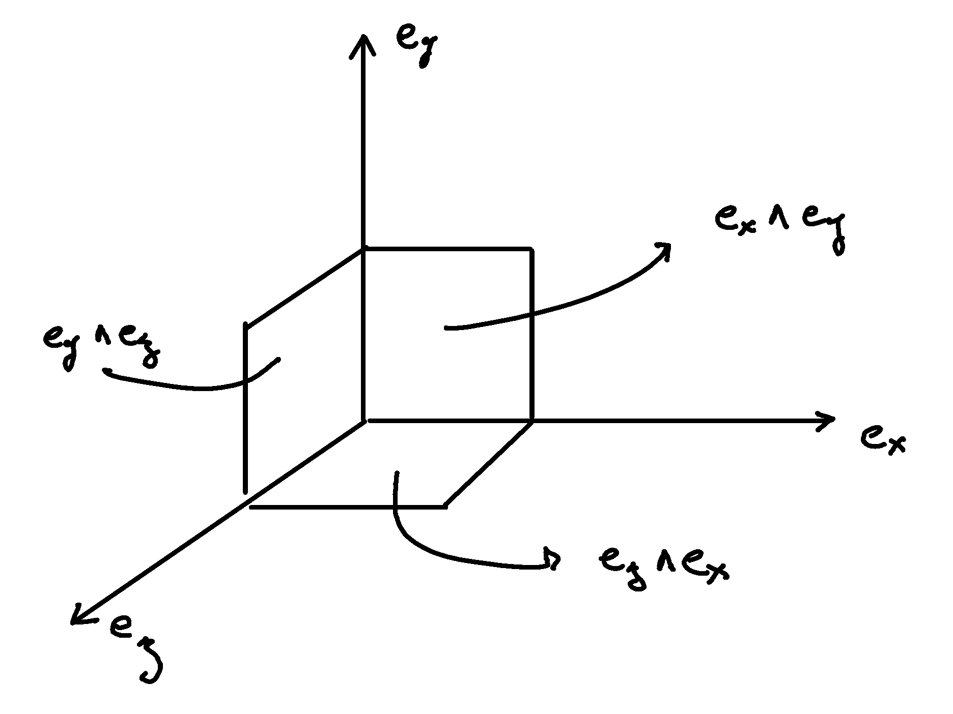
We notice we have also defined three planes:

• \(∂_y ∧ ∂_z\)

• \(∂_z ∧ ∂_x\)

• \(∂_x ∧ ∂_z\)

Where the wedge symbol \(∧\) denotes the surface spanned by two directions \(∂_i ∧ ∂_j\). The naming of the surfaces is carefully chosen counterclock wise. Taking this one step further, we notice that we have defined the volume element as well:

• \(∂_x ∧ ∂_y ∧ ∂_z\)

Indeed, the Euclidean space necessitate the dot product, which permits to not only determine the projection of a vector onto another \(V^♯ \cdot W^♯ = V^i W^j δ_{ji} cos(θ)\), but also the surface of the parallelogram defined by these two vectors \(|V^♯ ∧ W^♯| = V^i W^j δ_{ji} sin(θ)\).

Orientation of Space

We label and order vectors by the letters \(x\), \(y\), and \(z\). Cycling counterclockwise, the sequences are:

• \(x\) to \(y\) to \(z\), or

• \(y\) to \(z\) to \(x\), or

• \(z\) to \(x\) to \(y\)

Direction	Surface	Permutation
\(∂_x\)	\(∂_y ∧ ∂_z\)	\(x,y,z\)
\(∂_y\)	\(∂_z ∧ ∂_x\)	\(y,z,x\)
\(∂_z\)	\(∂_x ∧ ∂_z\)	\(z,x,y\)

Traversing the table above from left to right or top to bottom, we cycle through all permutations of the spatial directions. For a long time, I had difficulties with the term \(∂_z ∧ ∂_x\). My instinct was to order the elements of the basis bivectors alphabetically and thus take \(∂_x ∧ ∂_z\), but requires a negative sign when flipping the surface to \(-∂_z ∧ ∂_x\). Both conventions are correct but as can be read from the table, taking \(∂_z ∧ ∂_x\) is ultimately the superior choice.